Briomatic.com

Briomatic Technology is a SEO, Blog Management and Web Design company based out in Chennai and Dubai. Briomatic.com aim to support Small Medium Business (SMB) customer to achieve their sales with cost effective SEO, Web Design and Software Packages.

Briomatic IPL

 https://briomatic.com/ | www.tixs.ae | Plant Souq | Thiruvarur.in

Top Fantasy Cricket App in India

Are you looking to play your favourite fantasy cricket on Mobile app? Well, nowadays, most of us do not like to sit in front of the TV for the whole day not just watching only cricket. Well in the current scenario, we would like to watch cricket live but always most of us love to play fantacy cricket with good cricket apps.

Now, Cricket season is almost throughout the year. Millions of fans watch and play cricket on mobile. There is no better way to play you favourite fantasy cricket on your mobile phone or tablet today.

Altogether, fantasy cricket apps are also attracting too many people. And! Since the IPL 2022 has begun, the frenzy among the people is very high.

What is Fantasy Cricket?

Fantasy cricket, as the name suggests, is an online fantasy game where you can create a virtual cricket team of 11 players from an upcoming real-life match. The process of playing fantasy league cricket is quite simple. Your main objective is to score as many points as possible and achieve a position on the leadership board by beating your opponents on the fantasy cricket.

What is Fantasy Cricket Apps?

Fantasy cricket is a part of the Fantasy Sports. It is an online game where you create a virtual team of real cricket players and scores points depending on how your chosen players perform in real-life matches using the apps. It involves monetary risk as well.

Top 10 Fantasy Cricket App

Check out our article comprising a list of 10 Top Fantasy Cricket App for Android and iPhone to keep yourself the latest fantasy cricket app on the screen of your smartphone to play.

Here are the good fantacy cricket apps for both Android and iPhone in India

1# Dream11 Fantacy Cricket App

Play Online Fantasy Cricket on India’s Biggest Sports Platform. Dream11 is one of the most famous and widely used live fantasy cricket app available for Android and Apple. It is very easy to use and contains numerous features. Play Fantasy Cricket, Make your fantasy cricket team & win big.

Dream11 is one of the earliest apps in the fantasy world. With over 12 Crore players and 4.7 star rating, the Dream11 Fantasy Cricket App allows you to play various Cricket formats and challenge types using your cricketing skills. You can compete in various challenges to win amazing prizes. Dream 11 is a official partner and sponsor for Chennai Super Kings for IPL 2022 season.

2# My11Circle Fantasy Cricket App

My11Circle is a fantasy cricket app that lets users make a team of their own and create a strategy to win the fantasy game based on players they choose. My11Circle cricket fantasy website has started to gain more popularity in India among the online cricket players available in 9 different languages. BCCI director Saurav Ganguly is currently the brand ambassador of the My11Circle app.

My11Circle is a fantasy cricket app that lets users make a team of their own and create a strategy to win the fantasy game based on players they choose. Play Fantasy Cricket on My11Circle. Trusted by 1 Crore+ Players. My11Circle is an online fantasy sports game designed for fans who like to showcase their sports knowledge and analytical skills.

3# Mobile Premier League(MPL) Fantasy Cricket App

Mobile Premier League is the best fantasy sports app, the latest gaming platform with 4.6 rating. Play Fantasy Cricket on MPL & Win Daily Cash Prizes. Kohli had invested in Galactus Funware Technology, which owns Mobile Premier League (MPL). In November, 2020, BCCI announced MPL Sports – a brand from MPL – as its new kit sponsor.

The MPL fantasy app provides you with a seamless entry into the world of fantasy sports. With a user interface that is better than most other competitors in the region.

4# MyTeam11 Fantasy Cricket App

MyTeam11 can be found at the website of the Indian Federation of Sports Gaming (IFSG): www.ifsg.in. IFSG is recognized as India’s first and only self-regulatory sports gaming authority focusing on developing standardized practices in the industry.

MyTeam11 does not permit the users identified as the residents of Sikkim, Odisha, Telangana, Assam, Nagaland and Andhra Pradesh to participate in the pay-to-play contest(s) organized by MyTeam11.

Low commission leagues, fast & hassle free withdrawals, and less competition is what makes MyTeam11 worthy of all the popularity and affection

5# Fanfight Fantasy Cricket App

Fanfight App is also an online fantasy App or Website where you can earn real money by playing fantasy leagues. It is an fantasy game designed for fans who like to showcase their game knowledge and analytical skills.

Fanfight app is 100% real and genuine and it is one of the best fantasy apps in India. The withdrawal system is great and allows Withdrawl 

6# Gamezy Fantasy App

Play real fantasy game online app & win cash daily on Gamezy. Click now to learn everything about fantasy matches & get top tips to win every on gamezy app. Gamezy app is not like other Fantasy cricket league apps. This app helps to guaranteed cash reward and the winner get prize.

KL Rahul is the brand ambassador of the Gamezy Cricket Fantasy App. You can easily win IPL matches with the Gamezy app and can withdraw a minimum of Rs 200.

7# Howzat – Fantasy Cricket App

Howzat, the Best Fantasy Cricket App, can be downloaded on both kinds of devices – either Android or iOS. Play fantasy cricket game on Howzat app & win real cash.

Howzat is the ultimate fantasy cricket app for sports lovers. Get fantasy cricket match prediction, winning strategy, match schedules which covers complete details about IPL 2022.

Howzat, the fantasy cricket platform, is to partner with Legends League Cricket Oman, in their quest to bring the legends of cricket together and compete with each other for the ultimate prize. With a lineup of 45+ legends across 3 teams.

8# 11Wickets Fantasy App

11 wickets are a completely India based fantasy platform and projects itself as the all-desi platform.

11Wickets is one of the country’s fastest-growing fantasy platforms designed for users who run passionate about Cricket also which covers Kabaddi and football.

Coming Soon: Fantasy Cricket App Review, fantasy cricket app download, Features, Referral Code, Fantasy Cricket App  APK, FanFight Promo Code, Fantasy Cricket App Customer Care Number, Fantasy Cricket Apps win details will be available soon with complete review package for all the apps in India.

IPL Ticket | www.ipl.ae

IPL Cricket Blog: https://ipl.ae

Cricket is an emotion for the Indian cricket fans. To bring joy to the Cricket for fans of IPL, you can visit www.ipl.ae to get more updates and news on daily basis

Https://ipl.ae - The official Indian Premier League Fan Blog

Looking for Product or service from Etisalat? Please update your contact details and we will take care and call you back with your requirement.

Dubai - Just Visit

Interview Tips: 10 Attributes that employers WANT....‏

Adaptability: How good are you at dealing with change? We live in an
ever-changing world; the only certainty is that things will change. 
 
Commitment: All employers are looking for commitment in the people
they employ.
 
Communication: Can you show that you have an awareness of what
constitutes good lines of communication?
 
Creativity in Problem-Solving: Can you show that your approach to
solving problems does not rely on all the old familiar approaches?
 
Decision-Making: Be ready to give examples of a time when,
confronted with a problem or an opportunity, you examined the
options available and decided on an appropriate course of action. 
 
Evaluation: You need to show how you are committed to providing the
evaluation and review of the decisions you have taken. 
 
Foresight: How did you demonstrate the ability to see the trouble a
long way off before it was upon you? 
 
Independence: How much do you need to be supervised? Can you work on
your own? 
 
Team Player: organisations will want to see that you can lead and be
led - negotiate with others - work collaboratively on problems and
encourage colleagues to give their best.
 
Value-Added Marketing: You may not be a sales person but every
member of the organisation is expected to play a part in 'selling
the product'.
 

VLOOKUP in Excel – The Greatest Guide

VLOOKUP in Excel – The Massive Guide

VLOOKUP is one of the most useful and important functions in Microsoft Excel. It is generally used to look up a particular value in huge data sheets where manual intervention can be cumbersome. The alphabet ‘V’ in VLOOKUP stands for “Vertical” so this function is sometimes also called vertical lookup.
The term “Vertical” signifies that it can be used to look up values vertically i.e. it can be used to look up values inside a column.
You can also read my previous post: “How to alphabetize in Excel”, there I have used VLOOKUP for sorting a list.
Note: This is a long post over 2500+ words, you will feel comfortable navigating it the using below jump links.

• Definition of VLOOKUP in Excel
• What are the uses of Vertical Lookup Function?
• Syntax of VLOOKUP Function
• Few Important points about Vertical Lookup function
• How to Use VLOOKUP?
• 5 Beginner level examples of VLOOKUP function
• Few Practical Examples of Vertical Lookup function
• How to Use VLOOKUP in VBA
• How to return multiple columns from a VLOOKUP
• Negative VLOOKUP
• Creating a multiple criteria VLOOKUP

Definition of VLOOKUP in Excel:

According to Microsoft Excel VLOOKUP can be defined as a function, “that looks for a value in the leftmost column of a table, and then returns a value in the same row from a column you specify. By default the table must be sorted in an ascending order.”

What are the uses of Vertical Lookup Function?

This function is mostly used for following tasks:

1. To look up a single or a set of values from a data sheet.
2. To add a column to a datasheet from some other table, based on some unique (attribute)s.

Syntax of VLOOKUP Function:

Its syntax is as follows:

=VLOOKUP( lookup_value, table_array, column_index, range_lookup )

Here, ‘lookup_value’ specifies the value to be searched inside the ‘table_array’. It can either be a value or a reference.
‘table_array’ is the range with two or more columns. ‘table_array’ argument can receive a range reference or a named range. The leftmost column of this range must contain the ‘lookup_value’.
‘column_index’ is the relative index of the column whose value needs to be returned by the VLOOKUP function. A ‘column_index’ 1 would return values from the first column in the ‘table_array’ similarly ‘column_index’ 2 would return values from the second column in the ‘table_array’.
‘range_lookup’ is a Boolean value that specifies whether you want VLOOKUP to find an exact match or an approximate match. If its value is ‘True’ then either an approximate or an exact match will be returned. Here, if an exact match is not found, the next value that is less than ‘lookup_value’ is returned. If its value is ‘False’ then only exact match will be returned.

Few Important points about Vertical Lookup function:

• VLOOKUP function performs a case-insensitive lookup.
• VLOOKUP in Excel returns a ‘#N/A’ if it is not able to find the ‘lookup_value’ inside the ‘table_array’.
• It returns a ‘#VALUE!’ error if the value of ‘column_index’ is less than 1.
• It returns a ‘#REF!’ error if the value of ‘column_index’ is greater than the number of columns in the ‘table_array’.
• The default value of ‘range_lookup’ is TRUE. So, it is better to omit this argument in case you need to perform either an approximate or an exact match.
• Vertical Lookup allows you to use wildcard characters in the ‘lookup_value’ argument. We will discuss it later in this article.

How to Use VLOOKUP?

Before understanding how to use Vertical Lookup function, you must understand what its objective is. Let’s try to understand this with a sample problem.
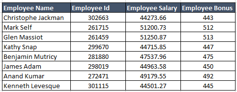
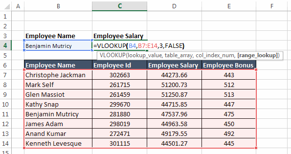
Suppose we have a table as shown below.

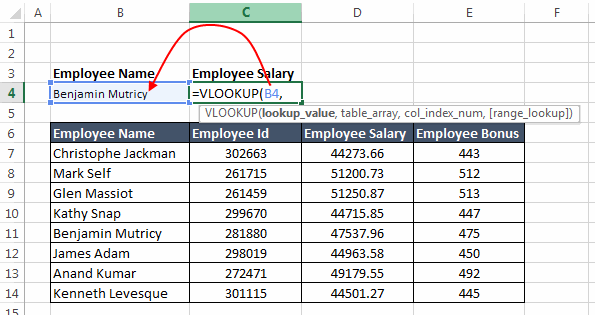
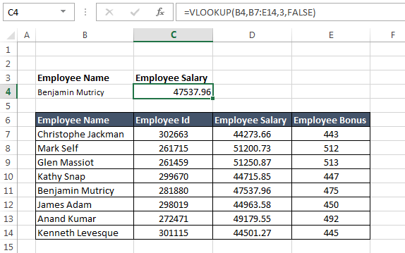
Objective: Our objective is to find the salary of any particular employee (say: Benjamin Mutricy) based on his name.
Solution: Now, lets try to apply a VLOOKUP to find the solution.

lookup_value: This is the value based on which the lookup is to be performed. In our case lookup_value is in the cell B4 i.e.  “Benjamin Mutricy”.

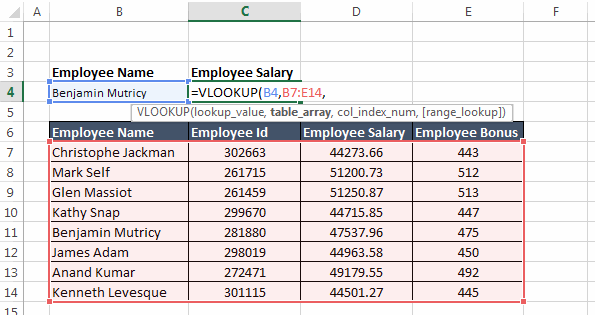
table_array: This is the range of the table from which the values are to be fetched. Note that this ‘table_array’ should always contain ‘lookup_value’ in its leftmost column.

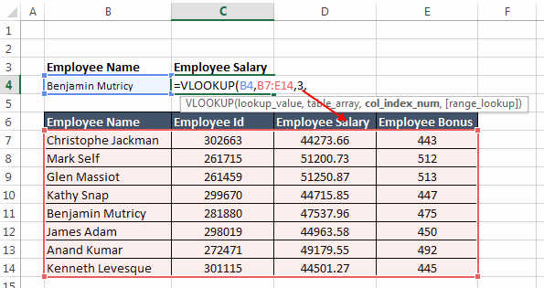
col_index_num: This specifies the positional reference of the column that you want the VLOOKUP to return.

range_lookup: This specifies that weather the match should be exact or approximate. FALSE specifies exact match.

So, in this case the VLOOKUP function would be: =VLOOKUP(B4,B7:D14,3,FALSE)

5 Beginner level examples of VLOOKUP function:

Now let’s move to some examples:
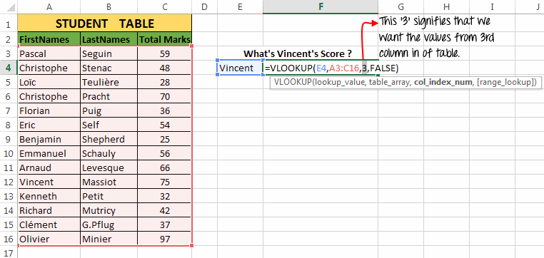
Example 1: In this example we have a list of students with their scores. Now, here we need to find the score of a student with the First Name ‘Vincent’.

To find the solution to our problem, we have used the vertical lookup as:
=VLOOKUP(E4,A3:C16,3,FALSE) and it gives the result 75.
Explanation:

• The first argument to the function i.e. ‘lookup_value’ = E4 (Reference of “Vincent”)
• Second argument i.e. ‘table_array’ = A3:C16 (Range of student table)
• Third argument i.e. ‘column_index’ = 3 (the column number whose value the VLOOKUP function should return)
• Fourth argument i.e. ‘range_lookup’ = FALSE (Signifies that we only want the exact match)

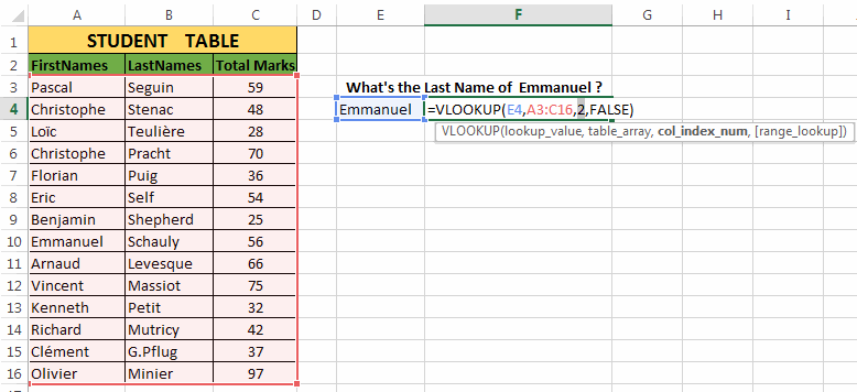
Example 2: In the next example we have the same table, but now our task is to find the last name of a student ‘Emmanuel’.

So, we will use the VLOOKUP as: =VLOOKUP(E4,A3:C16,2,FALSE) and it results into “Schauly”
Explanation:

• The first argument to the function i.e. ‘lookup_value’ = E4 (Reference of “Emmanuel”)
• Second argument i.e. ‘table_array’ = A3:C16 (Range of student table)
• Third argument i.e. ‘column_index’ = 2 (the column number whose value the VLOOKUP function should return)
• Fourth argument i.e. ‘range_lookup’ = FALSE (Signifies that we only want the exact match)

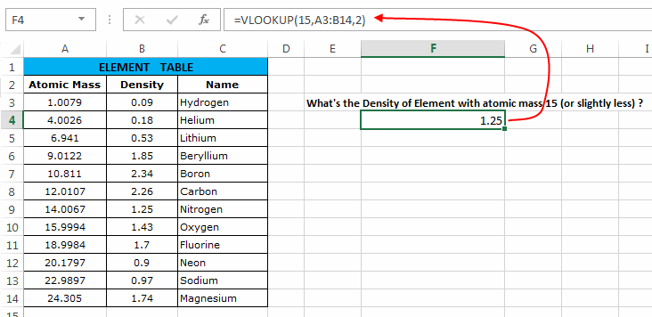
Example 3: In this example we have an “Element Table” table. The table contains 3 columns namely Atomic Mass, Density and Element Name.

Here we have to find the Density of an Element whose atomic mass is 15 or slightly less.
Now, here we can use the vertical lookup formula as: =VLOOKUP(15,A3:B14,2) which results into 1.25.
Explanation:

• The first argument to the function i.e. ‘lookup_value’ = 15 (Atomic Mass to be searched)
• Second argument i.e. ‘table_array’ = A3:B14 (Range of Element Table)
• Third argument i.e. ‘column_index’ = 2 (the column number whose value the vertical lookup function should return)
• Fourth argument i.e. ‘range_lookup’ is omitted and hence its value is true. So, first it searches 15 in the Atomic Mass column but when it fails to find 15, it returns the density of element slightly less than 15.

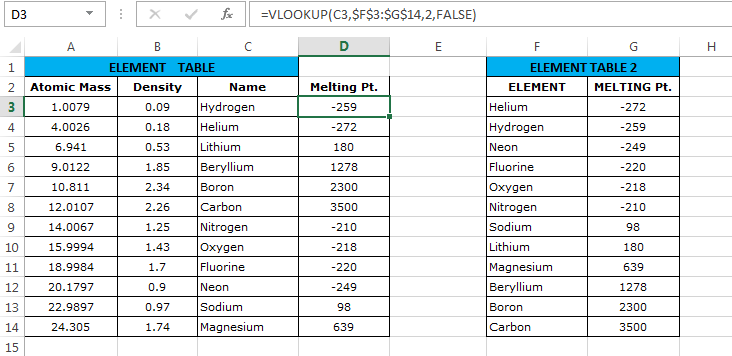
Example 4: In this example we have 2 tables as shown below. Our task is to apply a Vertical Lookup based on ‘Element Names’ and fetch the melting points of the elements from the second table.

This can be done by using the formula: =VLOOKUP(C3,$F$3:$G$14,2,FALSE)
After applying this formula for the first element we have to drag the formula below (using the fill handle) for other elements.
Explanation:

• The first argument to the function i.e. ‘lookup_value’ = C3 (Reference for first element)
• Second argument i.e. ‘table_array’ = $F$3:$G$14 (Range of Element Table 2) – If you are wondering what are these ‘$’ signs along with the table reference, then you should read this post.
• Third argument i.e. ‘column_index’ = 2 (the column number whose value the vertical lookup function should return)
• Fourth argument i.e. ‘range_lookup’ = FALSE (Signifies that we only want the exact match)

Note that the values that I have explained above are only for the first element. Dragging this formula itself makes the necessary changes in the formula to make it correct for the below elements as well.
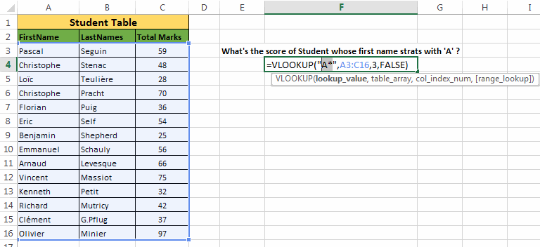
Example 5: In this example we will use wildcard operators along with Vertical Lookup. Here we have to find the score of the student whose first name starts with ‘A’.

For this we can use the formula: =VLOOKUP("A*",A3:C16,3,FALSE) which gives a result 66.
Explanation:
Generally, we can use following two wildcard operators with VLOOKUP function.

Wildcard	Description
‘?’	Denotes any single character.
‘*’	Denotes any number of characters

Note: Simply placing the tilde sign (~) before any wildcard character tells Excel that the wildcard character (‘*’ or ‘?’) should be treated as a string and not as wildcard operator.

• The first argument to the function i.e. ‘lookup_value’ = “A*” (Any word starting with ‘A’ alphabet)
• Second argument i.e. ‘table_array’ = A3:C16 (Range of Student Table)
• Third argument i.e. ‘column_index’ = 3 (the column number whose value the vertical lookup function should return)
• Fourth argument i.e. ‘range_lookup’ = FALSE (Signifies that we only want the exact match)

Few Practical Examples of Vertical Lookup function:

Now let’s see some practical examples of VLOOKUP Function:
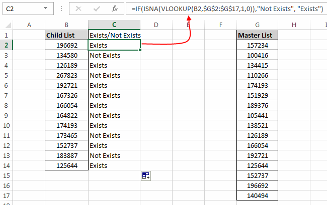
Example 6: Let’s say we have a list named “Child List” and another list with the name “Master list”. Now, using Vertical lookup we need to find if all the items in “Child List” are also present in the “Master list”.

In such a case we will use the formula: =IF(ISNA(VLOOKUP(B2,$G$2:$G$17,1,0)),"Not Exists", "Exists")
This formula uses If Statement, ISNA function and VLOOKUP.
Explanation:
Here IF statement checks whether the output of VLOOKUP function is #NA Error or not. IF the output is #NA error, then it means that current child list item is not present in the master list. And hence the IF statement writes “Not Exists” in front of it, however if the item is present in the master list then it writes “Exists”.
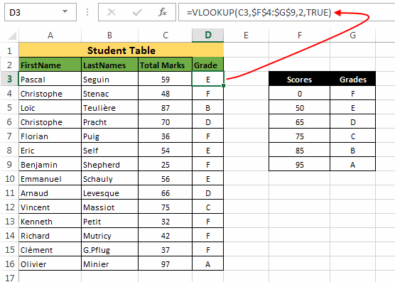
Example 7: Translating scores to grades using vertical lookup. Let’s say we have a table with student scores and now we have to assign them a grade based on their scores.

For this we can use a VLOOKUP as: =VLOOKUP(C3,$F$4:$G$9,2,TRUE) and then drag this formula to below cells.
Explanation:

• The first argument to the function i.e. ‘lookup_value’ = C3 (Reference for first element)
• Second argument i.e. ‘table_array’ = $F$4:$G$9 (Range of scores and grades table)
• Third argument i.e. ‘column_index’ = 2 (the column number whose value the VLOOKUP function should return)
• Fourth argument i.e. ‘range_lookup’ = True (It matches both the exact values and values slightly lesser)

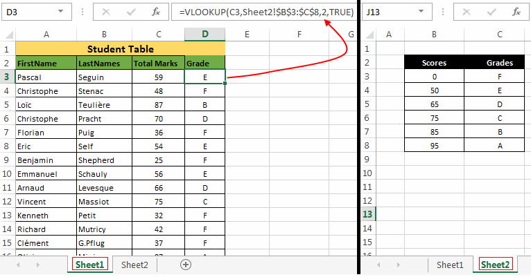
Example 8: Applying Vertical lookup using a table on another sheet or another workbook. In all the examples that we have discussed till now, we have applied VLOOKUP on tables that are on same worksheet. Now let’s redo the task in previous example but this time with the scores and grade table present on another worksheet sheet.

In this example the “Student Table” is on ‘Sheet1’ while the “Grade and Score table” is on the ‘Sheet2’. So you can use a VLOOKUP as: =VLOOKUP(C3,Sheet2!$B$3:$C$8,2,TRUE)
Explanation:

• The first argument to the function i.e. ‘lookup_value’ = C3 (Reference for first element)
• Second argument i.e. ‘table_array’ = Sheet2!$B$3:$C$8 (Range of scores and grades table which is present on Sheet2)
• Third argument i.e. ‘column_index’ = 2 (the column number whose value the vertical lookup function should return)
• Fourth argument i.e. ‘range_lookup’ = True (It matches both exact and values slightly lesser)

Tip: While writing such VLOOKUP formula you can simply navigate to the Sheet where the table is present and then select the required table. This will automatically insert the reference of that particular table in VLOOKUP formula.
See the below animation for more details:

How to Use VLOOKUP in VBA:

VLOOKUP function can also be used in VBA. Below is a sample code:

view plaincopy to clipboardprint?

1. Sub Vertical_lookup_test()  
2. Dim Result As Variant  
3. Dim myVal As String ' Can be Integer, long, double etc.  
4. Dim Rng As Range  
5. Dim Clm As Integer  
6. Set Rng = ActiveSheet.Range("A:E") ' Set Range  
7. myVal = "Florian" ' Value to be searched  
8. Clm = 3 ' Column to be fetched  
9. Result = Application.VLookup(myVal, Rng, Clm, False)  
10. If IsError(Result) Then  
11.   Result = "Not found!"  
12. End If  
13. MsgBox Result  
14. End Sub  

Before using the above code make sure you change the following values:
1. Change Set Rng = ActiveSheet.Range("A:E") to the range that you wish to use.
2. Change myVal = "Florian" to the value that you want the vertical lookup to search. You can also use the InputBox function to get this value from user during the runtime.
3. Change Clm = 3 to the column that you the VLOOKUP to fetch.

How to return multiple columns from a VLOOKUP?

Till now we have seen VLOOKUP functions that only returns a single column. But there are times when you need a VLOOKUP function to return multiple columns from the specified row.
So, you have to make a VLOOKUP formula that can fetch multiple columns. The basic idea behind this is, we will use VLOOKUP as an array function.
Follow the below steps to use this:
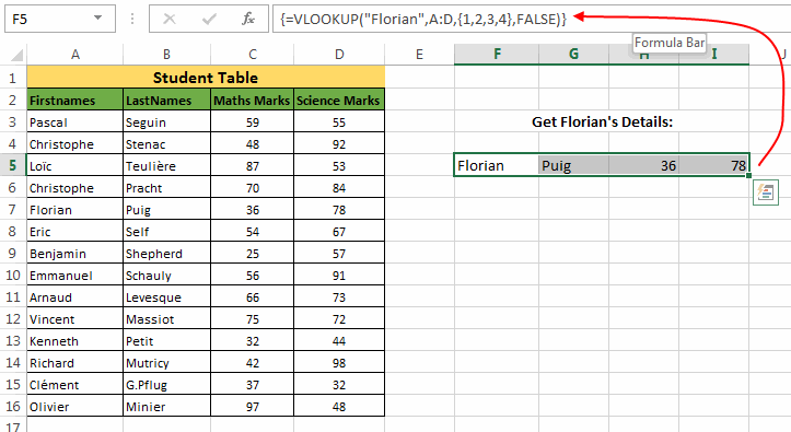
Suppose we need to fetch all the details of “Florian” so we will proceed as:
1. Select the cells (cells equal to the number of columns that you wish to fetch) where you wish to populate the VLOOKUP results.
2. Next, without clicking anywhere else type the formula: VLOOKUP("Florian",A:D,{1,2,3,4},FALSE) in the Formula bar. The third argument i.e. {1,2,3,4} specifies the columns that need to be fetched.

3. After this simply hit the Ctrl + Shift + Enter keys. This will enclose the above formula in curly brackets and the cells that you had selected will show the fetched columns.

Negative VLOOKUP:

In all the previous examples you must have seen that we have always used a ‘lookup_value’ that is present in the leftmost column of the range. So, the question arises, can we use a ‘lookup_value’ which is not in the leftmost column?

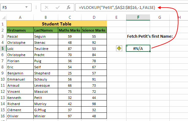
See what happens when your ‘lookup_value’ is not on the leftmost side, and you enter a negative ‘column_index’ hoping to fetch the value to the left of ‘lookup_value’.
A simple way to do this is by building a user defined function (UDF). This function internally doesn’t use VLOOKUP but it can give you desired results. Below is the UDF:

view plaincopy to clipboardprint?

1. Function NEGATIVE_VLOOKUP(lookup_value, table_array As Range, col_index_num As Integer, CloseMatch As Boolean)  
2. Dim RowNbr As Long  
3. RowNbr = Application.WorksheetFunction.Match(lookup_value, table_array.Resize(, 1), CloseMatch)  
4. NEGATIVE_VLOOKUP = table_array(RowNbr, 1).Offset(0, col_index_num)  
5. End Function  

This UDF uses Match and Offset functions to accomplish the task.
How to use this Negative VLOOKUP UDF:
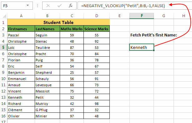
Let’s understand how to use this function. In our example we have a Student Table and we have to find the first name of “Petit”.
So, we will use this formula as: =NEGATIVE_VLOOKUP("Petit",B:B,-1,FALSE)

Explanation:

• The first argument to this UDF is the ‘lookup_value’.
• Second argument is the range where this UDF should search for ‘lookup_value’.
• Third argument is the positional reference of the column which this UDF should return.
• Last argument is the Boolean value specifying exact or approximate match.

Similarly, in the same table if we have to find the first name of the student with 98 Marks in Science, then the formula would be:
=NEGATIVE_VLOOKUP(98,D:D,-3,FALSE)

Creating a multiple criteria VLOOKUP:

While doing data analysis in excel sometimes you may run into situations where you need to apply a VLOOKUP based on two keys (i.e. based on two ‘lookup_values’).
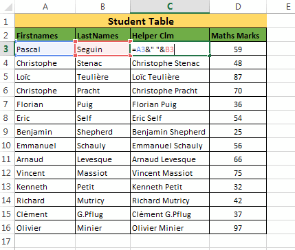
For example: We have a Student table as shown in the below image. Now, as you can see that there are two students with First Name “Christophe” (at A4 and A6). So, applying a VLOOKUP on first name can cause inconsistency. Hence we will apply a VLOOKUP based on both First name as well as the Last name.
But as we know that VLOOKUP in Excel can only have a single ‘lookup_value’. So we need to create a helper column by appending first name and last name as =A3&" "&B3

Now, we have combined two keys together and hence this new key column would contain unique values.

Next, we can simply apply a Vertical lookup as: =VLOOKUP("Christophe Pracht",C:D,2,FALSE)
So, this was all about VLOOKUP in Excel. Do read this post if this long article has bored you and don’t forget to share your ideas and thoughts with us in the comments section.

Inspirational Story - Heart Touching One - True Motivation

How to Apply for a Passport In India!!!

 

1. Get the Passport Application Form: One can apply for Passport through Online Registration, (after doing online registration, get print outs of the application form) click here for details for Online Registration. Apart from this applicant can submit directly in the respective passport office/ DPCs/Speed post centers, get the relevant application form from here.

2. How to fill the Form: The Passport Application Form is Machine Readable. Please follow the instructions as follows:

    Use capital letters only. Particulars given in the form will be printed in the passport. Therefore, please be careful in filling up the form and avoid any mistakes.

    Use black/blue ball pen only

    Do not fill the form with pencils or ink-pen.

    While filling up the boxes, kindly leave one box blank after each completed word.

    Write clearly within the box without touching the boundaries.

    Adjust the information to fit within the number of given boxes.

    Do not write anything outside the box.  Avoid over-writing

    Incomplete application will not be accepted.

Columnwise Guidelines for filling the application form can be had from here.

Note:   All original documents are to be shown at the time of submission of the passport application form. With the Original Passport Application Form, self-attested copies of all required documents need to be attached. Illiterate applicants should put only thumb impression in the box meant for thumb impression/signature. In case an applicant has stayed at more than one address during the last one year, he/she should furnish two additional photocopies of the PP form for each additional place of stay.

3. Where to Apply : For Online Registration, the applicant has to submit the print outs of the application form along with required documents to the respective passport office in the appointment date and time printed. Apart from this Passport Applications can be submitted at

    The counter of the Passport office

    The Speed Post centers

    District Passport Cells

    Passport Collection Centers

An application for a passport may be submitted personally OR through a representative (any close member of the family or recognized travel agent(s) only) carrying an authority letter.

ONLINE APPLICATION:

JUST GO TO WEB: http://passport.gov.in/

CREATE THE PERSONAL LOGIN

DOWNLOAD APPLICATION TO APPLY ONLINE

FILL THE FORM

UPLOAD WITH THE UPDATED DETAILS IN THE FORM (xml Format)

Then

Apply for Appointment based on your location

Once you get the appointment page… Fix your appointment based on your convenient timing…

Then

Go to the respective passport Kendra with the supporting document with original and Photo copy… (1set)

No need of Photo…

It’s a simple process…. Everyone can do it personally. No need to get into Brokers or Agent!!!

IF YOU NEED ASSISTANCE … SEND A MAIL TO RIFAMAIL@GMAIL.COM

10 Step to Improve your Communication Skill

Communication Skills is a term used to describe a broad set of skills needed to achieve two simple objective - To transmit to oneself or someone else information with the required interpretation and understanding and​having yourself or that person feel they way you want them to feel in the process.

10 basic disciplines to master good communication skills are as follow:

1. Choose someone you think has good communication skills and imitate them till you master his or her skill. Then find another person with even better communication skills and raise your level even higher.

2. Hang out with people who have good communication skills. Hanging out with any lesser kind will have a negative impact on your communication skills.

3. Practice Oratory. Everyday, select a word or a sentence(eg news headlines) and talk to your self for 5 mins on that topic or anything related to it. The objective here is to be creative and spontaneous.

4. Read any book you lay your eyes on which will help you only get better.

5. When you are at public places, increase your sensory acuity by noticing peoples body language, lip-reading, and observing they behavior ie the way they interact with other people. Those very skills will help you analyze those you communicate with.

6. Set the objective to be nice to every person you meet, no matter what their attitude towards you is. Attitude is contagious.

7. Set the objective of every meeting, even if you meet a person unexpectedly.



If you are meeting a friend just to hand out, ask yourself "how do i want to feel at the end of it? How do i want to make my friend feel?" If you want to have fun - say it "For the next hour, i just want to have fun"

8. When communicating with a single person or a group, let the other person talk (and you listen) most of the time. People like to hear but love to be heard.

9. Good Communication Skills begin at home. Therefore, the previous 3 steps must first be applied while communicating with family members.

10. Before going to bed, take a minute and review the day. How well did you communicate with people today? How could you have improved the response/result?

Success is a few daily disciplines practiced everyday, so practice these steps daily and in few weeks you'll find vast improvements in the way people respond to you.

ESPN Legends of Cricket

Top 25 Cricketers Of All Time

1. Don Bradman
2. Gary Sobers
3. Viv Richards
4. Shane Warne
5. Jack Hobbs
6. Dennis Lillee
7. Sachin Tendulkar
8. Imran Khan
9. Wally Hammond
10. Sunny Gavaskar
11. Ian Botham
12. Richards Hadlee
13. Keith Miller
14. W.G. Grace
15. Graeme Pollock
16. Malcolm Marshall
17. Greg Chappell
18. George Headley
19. Frank Worrell
20. Len Hutton
21. Wasim Akram
22. Kapil Dev
23. Steve Waugh
24. Barry Richards
25. Allan Border

Living Legend Sachin in the 7th Place... 

Who told that "the people those who created History - They can't read their own"

Sachin - Changed the History!!!

Proud to be a Fan of Sachin!!!!

www.rifamail.blogspot.in

MEDICAL BILLING - INFO FOR THE DAY!

MEDICARE HEALTH IDENTIFIER NUMBER SUFFIXES ------------------------------------------ B = AGED WIFE, AGE 62 OR OVER (1ST CLAIMANT) B1 = AGED HUSBAND, AGE 62 OR OVER (1ST CLAIMANT) B2 = YOUNG WIFE, WITH A CHILD IN HER CARE (1ST CLAIMANT) B3 = AGED WIFE (2ND CLAIMANT) B4 = AGED HUSBAND (2ND CLAIMANT) B5 = YOUNG WIFE (2ND CLAIMANT) B6 = DIVORCED WIFE, AGE 62 OR OVER (1ST CLAIMANT) 1 VITAL STATISTICS RECORD POSITIONS NAME TYPE LENGTH BEG END CONTENTS --------------------------- ---- ------ --------- ------------------------------------------------------ B7 = YOUNG WIFE (3RD CLAIMANT) B8 = AGED WIFE (3RD CLAIMANT) B9 = DIVORCED WIFE (2ND CLAIMANT) BA = AGED WIFE (4TH CLAIMANT) BD = AGED WIFE (5TH CLAIMANT) BG = AGED HUSBAND (3RD CLAIMANT) BH = AGED HUSBAND (4TH CLAIMANT) BJ = AGED HUSBAND (5TH CLAIMANT) BK = YOUNG WIFE (4TH CLAIMANT) BL = YOUNG WIFE (5TH CLAIMANT) BN = DIVORCED WIFE (3RD CLAIMANT) BP = DIVORCED WIFE (4TH CLAIMANT) BQ = DIVORCED WIFE (5TH CLAIMANT) BR = DIVORCED HUSBAND (1ST CLAIMANT) BT = DIVORCED HUSBAND (2ND CLAIMANT) BW = YOUNG HUSBAND (2ND CLAIMANT) BY = YOUNG HUSBAND (1ST CLAIMANT) C1-C9,CA-CK = CHILD (INCLUDES MINOR, STUDENT OR DISABLED CHILD) D = AGED WIDOW, 60 OR OVER (1ST CLAIMANT) D1 = AGED WIDOWER, AGE 60 OR OVER (1ST CLAIMANT) D2 = AGED WIDOW (2ND CLAIMANT) D3 = AGED WIDOWER (2ND CLAIMANT) Page 2 of 12 VTLSTAT 8/29/2002 http://hcfanet.hcfa.gov/hpages/ois/metadata/dataadmn/RIF/VTLSTAT.HTM D4 = WIDOW (REMARRIED AFTER ATTAINMENT OF AGE 60) (1ST CLAIMANT) D5 = WIDOWER (REMARRIED AFTER ATTAINMENT OF AGE 60) (1ST CLAIMANT) D6 = SURVIVING DIVORCED WIFE, AGE 60 OR OVER (1ST CLAIMANT) D7 = SURVIVING DIVORCED WIFE (2ND CLAIMANT) D8 = AGED WIDOW (3RD CLAIMANT) D9 = REMARRIED WIDOW (2ND CLAIMANT) DA = REMARRIED WIDOW (3RD CLAIMANT) DD = AGED WIDOW (4TH CLAIMANT) DG = AGED WIDOW (5TH CLAIMANT) DH = AGED WIDOWER (3RD CLAIMANT) DJ = AGED WIDOWER (4TH CLAIMANT) DK = AGED WIDOWER (5TH CLAIMANT) DL = REMARRIED WIDOW (4TH CLAIMANT) DM = SURVIVING DIVORCED HUSBAND (2ND CLAIMANT) DN = REMARRIED WIDOW (5TH CLAIMANT) DP = REMARRIED WIDOWER (2ND CLAIMANT) DQ = REMARRIED WIDOWER (3RD CLAIMANT) DR = REMARRIED WIDOWER (4TH CLAIMANT) DS = SURVIVING DIVORCED HUSBAND (3RD CLAIMANT) DT = REMARRIED WIDOWER (5TH CLAIMANT) DV = SURVIVING DIVORCED WIFE (3RD CLAIMANT) DW = SURVIVING DIVORCED WIFE (4TH CLAIMANT) DX = SURVIVING DIVORCED HUSBAND (4TH CLAIMANT) DY = SURVIVING DIVORCED WIFE (5TH CLAIMANT) 1 VITAL STATISTICS RECORD POSITIONS NAME TYPE LENGTH BEG END CONTENTS --------------------------- ---- ------ --------- ------------------------------------------------------ DZ = SURVIVING DIVORCED HUSBAND (5TH CLAIMANT) E = MOTHER (WIDOW) (1ST CLAIMANT) E1 = SURVIVING DIVORCED MOTHER (1ST CLAIMANT) E2 = MOTHER (WIDOW) (2ND CLAIMANT) E3 = SURVIVING DIVORCED MOTHER (2ND CLAIMANT) E4 = FATHER (WIDOWER) (1ST CLAIMANT) Page 3 of 12 VTLSTAT 8/29/2002 http://hcfanet.hcfa.gov/hpages/ois/metadata/dataadmn/RIF/VTLSTAT.HTM E5 = SURVIVING DIVORCED FATHER (WIDOWER) (1ST CLAIMANT) E6 = FATHER (WIDOWER) (2ND CLAIMANT) E7 = MOTHER (WIDOW) (3RD CLAIMANT) E8 = MOTHER (WIDOW) (4TH CLAIMANT) E9 = SURVIVING DIVORCED FATHER (WIDOWER) (2ND CLAIMANT) EA = MOTHER (WIDOW) (5TH CLAIMANT) EB = SURVIVING DIVORCED MOTHER (3RD CLAIMANT) EC = SURVIVING DIVORCED MOTHER (4TH CLAIMANT) ED = SURVIVING DIVORCED MOTHER (5TH CLAIMANT EF = FATHER (WIDOWER) (3RD CLAIMANT) EG = FATHER (WIDOWER) (4TH CLAIMANT) EH = FATHER (WIDOWER) (5TH CLAIMANT) EJ = SURVIVING DIVORCED FATHER (3RD CLAIMANT) EK = SURVIVING DIVORCED FATHER (4TH CLAIMANT) EM = SURVIVING DIVORCED FATHER (5TH CLAIMANT) F1 = FATHER F2 = MOTHER F3 = STEPFATHER F4 = STEPMOTHER F5 = ADOPTING FATHER F6 = ADOPTING MOTHER F7 = SECOND ALLEGED FATHER F8 = SECOND ALLEGED MOTHER J1 = PRIMARY PROUTY ENTITLED TO HIB (LESS THAN 3 Q.C.) (GENERAL FUND) J2 = PRIMARY PROUTY ENTITLED TO HIB (OVER 2 Q.C.) (RSI TRUST FUND) J3 = PRIMARY PROUTY NOT ENTITLED TO HIB (LESS THAN 3 Q.C.) (GENERAL FUND) J4 = PRIMARY PROUTY NOT ENTITLED TO HIB (OVER 2 Q.C.) (RSI TRUST FUND) K1 = PROUTY WIFE ENTITLED TO HIB (LESS THAN 3 Q.C.) (GENERAL FUND) (1ST CLAIMANT) K2 = PROUTY WIFE ENTITLED TO HIB (OVER 2 Q.C.) (RSI TRUST FUND) (1ST CLAIMANT) K3 = PROUTY WIFE NOT ENTITLED TO HIB (LESS Page 4 of 12 VTLSTAT 8/29/2002 http://hcfanet.hcfa.gov/hpages/ois/metadata/dataadmn/RIF/VTLSTAT.HTM THAN 3 Q.C.) (GENERAL FUND) (1ST 1 VITAL STATISTICS RECORD POSITIONS NAME TYPE LENGTH BEG END CONTENTS --------------------------- ---- ------ --------- ------------------------------------------------------ CLAIMANT) K4 = PROUTY WIFE NOT ENTITLED TO HIB (OVER 2 Q.C.) (RSI TRUST FUND) (1ST CLAIMANT) K5 = PROUTY WIFE ENTITLED TO HIB (LESS THAN 3 Q.C.) (GENERAL FUND) (2ND CLAIMANT) K6 = PROUTY WIFE ENTITLED TO HIB (OVER 2 Q.C.) (RSI TRUST FUND) (2ND CLAIMANT) K7 = PROUTY WIFE NOT ENTITLED TO HIB (LESS THAN 3 Q.C.) (GENERAL FUND) (2ND CLAIMANT) K8 = PROUTY WIFE NOT ENTITLED TO HIB (OVER 2 Q.C.) (RSI TRUST FUND) (2ND CLAIMANT) K9 = PROUTY WIFE ENTITLED TO HIB (LESS THAN 3 Q.C.) (GENERAL FUND) (3RD CLAIMANT) KA = PROUTY WIFE ENTITLED TO HIB (OVER 2 Q.C.) (RSI TRUST FUND) (3RD CLAIMANT) KB = PROUTY WIFE NOT ENTITLED TO HIB (LESS THAN 3 Q.C.) (GENERAL FUND) (3RD CLAIMANT) KC = PROUTY WIFE NOT ENTITLED TO HIB (OVER 2 Q.C.) (RSI TRUST FUND) (3RD CLAIMANT) KD = PROUTY WIFE ENTITLED TO HIB (LESS THAN 3 Q.C.) (GENERAL FUND) (4TH CLAIMANT) KE = PROUTY WIFE ENTITLED TO HIB (OVER 2 Q.C (4TH CLAIMANT) KF = PROUTY WIFE NOT ENTITLED TO HIB (LESS THAN 3 Q.C.)(4TH CLAIMANT) KG = PROUTY WIFE NOT ENTITLED TO HIB (OVER 2 Q.C.)(4TH CLAIMANT) KH = PROUTY WIFE ENTITLED TO HIB (LESS THAN 3 Q.C.)(5TH CLAIMANT) KJ = PROUTY WIFE ENTITLED TO HIB (OVER 2 Q.C.) (5TH CLAIMANT) KL = PROUTY WIFE NOT ENTITLED TO HIB (LESS THAN 3 Q.C.)(5TH CLAIMANT) Page 5 of 12 VTLSTAT 8/29/2002 http://hcfanet.hcfa.gov/hpages/ois/metadata/dataadmn/RIF/VTLSTAT.HTM KM = PROUTY WIFE NOT ENTITLED TO HIB (OVER 2 Q.C.) (5TH CLAIMANT) M = UNINSURED-NOT QUALIFIED FOR DEEMED HIB M1 = UNINSURED-QUALIFIED BUT REFUSED HIB T = UNINSURED-ENTITLED TO HIB UNDER DEEMED OR RENAL PROVISIONS TA = MQGE (PRIMARY CLAIMANT) TB = MQGE AGED SPOUSE (FIRST CLAIMANT) TC = MQGE DISABLED ADULT CHILD (FIRST CLAIMANT) TD = MQGE AGED WIDOW(ER) (FIRST CLAIMANT) TE = MQGE YOUNG WIDOW(ER) (FIRST CLAIMANT) TF = MQGE PARENT (MALE) TG = MQGE AGED SPOUSE (SECOND CLAIMANT) TH = MQGE AGED SPOUSE (THIRD CLAIMANT) TJ = MQGE AGED SPOUSE (FOURTH CLAIMANT) TK = MQGE AGED SPOUSE (FIFTH CLAIMANT) 1 VITAL STATISTICS RECORD POSITIONS NAME TYPE LENGTH BEG END CONTENTS --------------------------- ---- ------ --------- ------------------------------------------------------ TL = MQGE AGED WIDOW(ER) (SECOND CLAIMANT) TM = MQGE AGED WIDOW(ER) (THIRD CLAIMANT) TN = MQGE AGED WIDOW(ER) (FOURTH CLAIMANT) TP = MQGE AGED WIDOW(ER) (FIFTH CLAIMANT) TQ = MQGE PARENT (FEMALE) TR = MQGE YOUNG WIDOW(ER) (SECOND CLAIMANT) TS = MQGE YOUNG WIDOW(ER) (THIRD CLAIMANT) TT = MQGE YOUNG WIDOW(ER) (FOURTH CLAIMANT) TU = MQGE YOUNG WIDOW(ER) (FIFTH CLAIMANT) TV = MQGE DISABLED WIDOW(ER) FIFTH CLAIMANT TW = MQGE DISABLED WIDOW(ER) FIRST CLAIMANT TX = MQGE DISABLED WIDOW(ER) SECOND CLAIMANT TY = MQGE DISABLED WIDOW(ER) THIRD CLAIMANT TZ = MQGE DISABLED WIDOW(ER) FOURTH CLAIMANT T2-T9 = DISABLED CHILD (SECOND TO NINTH CLAIMANT) W = DISABLED WIDOW, AGE 50 OR OVER (1ST CLAIMANT) W1 = DISABLED WIDOWER, AGE 50 OR OVER (1ST CLAIMANT) W2 = DISABLED WIDOW (2ND CLAIMANT) W3 = DISABLED WIDOWER (2ND CLAIMANT) W4 = DISABLED WIDOW (3RD CLAIMANT) Page 6 of 12 VTLSTAT 8/29/2002 http://hcfanet.hcfa.gov/hpages/ois/metadata/dataadmn/RIF/VTLSTAT.HTM W5 = DISABLED WIDOWER (3RD CLAIMANT) W6 = DISABLED SURVIVING DIVORCED WIFE (1ST CLAIMANT) W7 = DISABLED SURVIVING DIVORCED WIFE (2ND CLAIMANT) W8 = DISABLED SURVIVING DIVORCED WIFE (3RD CLAIMANT) W9 = DISABLED WIDOW (4TH CLAIMANT) WB = DISABLED WIDOWER (4TH CLAIMANT) WC = DISABLED SURVIVING DIVORCED WIFE (4TH CLAIMANT) WF = DISABLED WIDOW (5TH CLAIMANT) WG = DISABLED WIDOWER (5TH CLAIMANT) WJ = DISABLED SURVIVING DIVORCED WIFE (5TH CLAIMANT) WR = DISABLED SURVIVING DIVORCED HUSBAND (1ST CLAIMANT) WT = DISABLED SURVIVING DIVORCED HUSBAND